Avoiding a Common Mistake in the Analysis of Repairable Systems

[Please note that the following article — while it has been updated from our newsletter archives — may not reflect the latest software interface and plot graphics, but the original methodology and analysis steps remain applicable.]

A system is a collection of subsystems, assemblies and/or components arranged in a specific design to achieve the desired functionality. A system can be repairable or non-repairable and the appropriate analysis method will differ based on this distinction. This article describes a mistake that is often made in repairable systems analysis (i.e., distribution analysis of times between failure) and presents two methods that are more appropriate for this type of analysis (i.e., analyzing system level data with a stochastic process model or analyzing component level data with a reliability block diagram). An example using race car field data demonstrates why distribution analysis of times between failure is not appropriate. This example is also used to highlight the advantages and disadvantages of the stochastic process model and reliability block diagram approaches.

Repairable Systems

A repairable system is a system that can be restored to an operating condition following a failure. Questions of interest in repairable systems analysis include:

How many failures will occur over a fixed time interval?
What is the probability of a failure in the next time interval?
What is the availability of the system?
How many spare parts should be purchased?
What is the cost of maintaining the system?
What is the optimum overhaul time?

Common Mistake When Analyzing Repairable Systems

One of the most common mistakes in analyzing repairable systems is fitting a distribution to the system's interarrival data. Interarrival data consists of the times between failure of a repairable system, as shown in the following picture where T_i is the cumulative time to failure and t_i is the interarrival time = T_i - T_i-1.

When fitting a distribution, we assume that the events are statistically independent and identically distributed (s.i.i.d.). However, in a repairable system, the events (failures) are not independent and in most cases are not identically distributed. When a failure occurs in a repairable system, the remaining components have a current age. The next failure event depends on this current age. Thus, the failure events at the system level are dependent.

When we perform a distribution analysis on the times between failure, this is equivalent to saying that we have 9 different systems, and System 1 failed after t₁ hours of operation, System 2 failed after t₂,…, etc.

Equation showing system failures

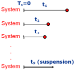
This is the same as assuming that the system is AS-GOOD-AS-NEW after the repair, which is not true in repairable systems in general. In most cases, the system is AS-BAD-AS-OLD after the repair. This is particularly true for large systems, where replacing a component does not have a great impact on the system reliability. For example, replacing the starter does not have a great impact on the reliability of a car since there are many other ways that it may fail.

Example: Will the Driver Finish the Race?

To demonstrate the problems with this analysis approach, consider the following example, which uses test data to analyze how a car will perform in a race. Each race is 200 Km. The brakes are changed after each race but all other components stay on the car for the next race. Table 1 displays data from three race cars operating under test. During the test, all vehicles operated under similar conditions and the brakes were preventively replaced every 305 Km. Note that the preventive maintenance (PM) interval for the brakes is longer in the test conditions than in the field so that the test specimens can be observed for a longer operating period.

Table 1: Field Data for 3 Race Cars

System 1 Age=2500 Km		System 2 Age=1976 Km		System 3 Age=800 Km
Time-to-Event	Component	Time-to-Event	Component	Time-to-Event	Component
249.8	Engine	305.0	PM Brakes	305.0	PM Brakes
305.0	PM Brakes	610.0	PM Brakes	453.9	Rear Suspension
584.2	Front Suspension	872.4	Engine	610.0	PM Brakes
610.0	PM Brakes	899.8	Right Front Brake	743.5	Transmission
915.0	PM Brakes	899.8	PM Brakes
972.0	Engine	1204.8	PM Brakes
1220.0	PM Brakes	1371.7	Right Front Brake
1525.0	PM Brakes	1371.7	PM Brakes
1830.0	PM Brakes	1470.4	Engine
1861.7	Front Suspension	1572.6	Rear Suspension
1994.6	Rear Suspension	1676.7	PM Brakes
2127.0	Transmission	1754.9	Transmission
2134.3	Right Rear Brake
2134.3	PM Brakes
2186.9	Engine
2439.3	PM Brakes

As shown in Figure 1, we could use Weibull++ to fit a distribution to the times between failure for each system. Note that the PM times are not considered and the time between the last failure and the current age of the system is treated as a suspension. This analysis assumes that we have a sample of 19 systems, and one system failed at 7.3 Km, another failed at 27.4 Km, and so on. The result is a 2-parameter Weibull distribution with beta = 1.1043 and eta = 336.7140. When you use this analysis to calculate the probability that the driver will finish the 200 Km race, the estimate is 56.97%. However, this result is not valid because the events (times between failure) are not s.i.i.d. When applied inappropriately, the analysis method yields incorrect results.

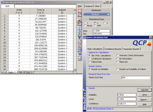
Figure 1: Distribution Analysis on Times Between Failure (in Weibull++)

Instead of fitting a distribution to the times between failure for each system, we could fit a distribution to the first time-to-failure for each system. These are statistically independent and identically distributed events. Figure 2 shows this analysis performed in Weibull++.

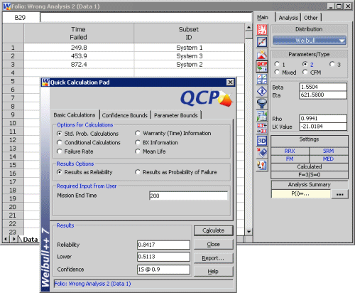
Figure 2: Distribution Analysis on First Time-to-Failure per System (in Weibull++)

The results from this type of analysis are limited, however. We could use this analysis to estimate the probability that the car will not fail in the first 200 Km (84.17%). But the confidence interval for this estimate is very wide (one-sided lower 90% bound = 51.13%). When we go on to estimate the probability that no failures will occur in the first ten races (2,000 Km), we find that the system will fail at least once in the next ten races (i.e., the reliability is 0%). However, we cannot use this analysis to estimate how many times the car will fail during the ten races. We also cannot determine whether and/or when to overhaul the system, and so on.

Clearly, a different analysis approach is required that will provide answers to these and other important questions. The remainder of this article presents two methods that are more appropriate for repairable systems analysis and considers the advantages and disadvantages of each method.

Using a Stochastic Process Model to Analyze Data at the System Level
For proper analysis of repairable systems, we need a model that will take into account the fact that the system has a current age whenever a failure occurs. For example, in System 1, the system has a current age of 249.8 Km after the engine is replaced. In other words, all other components in the system are 249.8 Km "old" and the next failure event will be based on this fact. Since the engine was just replaced, it is less likely to fail soon; whereas the failure probability for any of the other components is affected by the fact that they have already operated for 249.8 Km.

The Non Homogeneous Poisson Process (NHPP) with a Power Law Failure Intensity is such a model. It assumes that the system is AS-BAD-AS-OLD after each repair and is given by:

Where:

Pr[N(T)=n] is the probability that n failures will be observed by time T.
λ'(T) is the Failure Intensity Function (Rate of Occurrence of Failures).

NOTE: If we assume that the repair partially renews the system and it is not AS-BAD-AS-OLD after the repair, then the NHPP model may not be the most appropriate model for the analysis. The General Renewal Process (GRP) may be used instead.

Using the NHPP Power Law Model for the Race Car Analysis

As shown in Figure 3 and Figure 4, we can use ReliaSoft RGA software to apply the NHPP Power Law model to the race car data. This analysis estimates 6 failures per system over 10 races. With 2 cars in each race, that means we can expect 12 failures per fleet. If the average cost per failure is $192,000, then the total maintenance cost for the fleet is estimated to be: 12 Failures * $192,000/failure = $2,304,000.

NHPP Power Law Analysis (in RGA 6)

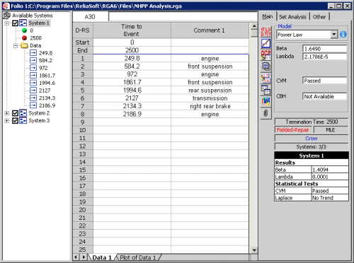
Figure 3: NHPP Power Law Analysis (in RGA 6)

Cumulative Number of Failures from the NHPP Analysis in RGA 6

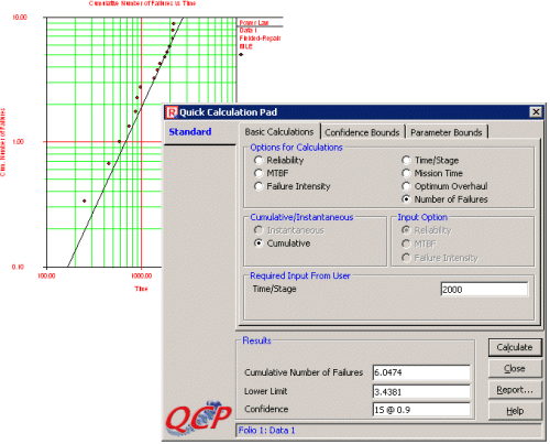
Figure 4: Cumulative Number of Failures from the NHPP Analysis in RGA 6

Using the Quick Calculation Pad, we can also estimate the probability that the driver will finish the first race (87.31%) and the probability that the driver will finish the third race given that his car has run the first two races, (66.70%). We can estimate the optimum overhaul time for the car by considering the average repair cost ($192,000) and the overhaul cost ($500,000). This is about 1,560 Km (approximately once every 8 races per vehicle). These results are shown in Figure 5.

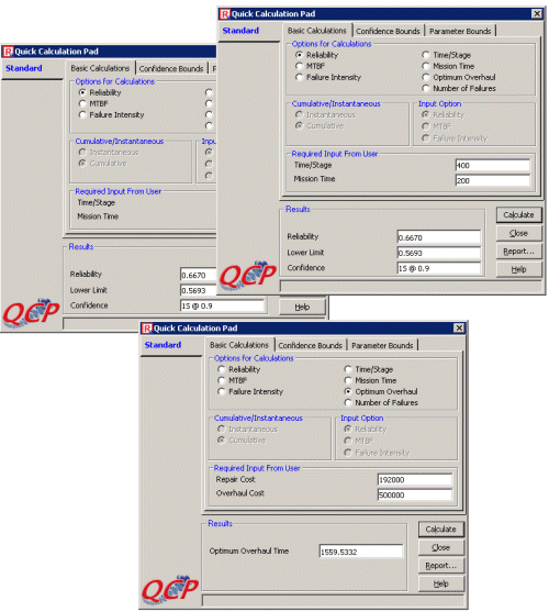
Probabilities of Finishing Race 1 and Race 3 and Optimum Overhaul Time (estimated in RGA 6)

Figure 5: Probabilities of Finishing Race 1 and Race 3 and Optimum Overhaul Time
(estimated in RGA 6)

As you can see, the NHPP analysis allows us to answer many questions of interest for a repairable system. However, there are still some unanswered questions, including:

How many spare parts should we purchase?
Which components cause most of the failures?
Can we get a more accurate cost estimate?

If we have data at the component level (Lowest Replaceable Unit, LRU), we can use a Reliability Block Diagram (RBD) approach to answer these and other questions.

Using an RBD for the Race Car Analysis

To use the race car example to demonstrate the RBD approach, let's assume that we have data for 6 replaceable components:

Engine
Transmission
Front & Rear Brakes
Front & Rear Suspension

We can use Weibull++ to analyze the times-to-failure and suspensions for each component. The results are shown in Table 2.

Table 2: Component Distributions and Parameters

Component	Distribution	Parameter 1	Parameter 2
Brakes Front L	Weibull	3.22	716.12
Brakes Front R	Weibull	3.22	716.12
Brakes Rear L	Weibull	15.36	391.41
Brakes Rear R	Weibull	15.36	391.41
Engine	Weibull	2.82	905.79
Front Suspension	Lognormal	7.29	0.65
Rear Suspension	Weibull	2.46	1564.36
Transmission	Weibull	3.14	1737.35

We can then use ReliaSoft's BlockSim software to create an RBD that represents the reliability-wise configuration of these components, as shown in Figure 6. We use the Weibull++ analyses to define the failure characteristics for each block in the diagram and also enter the repair durations and costs. For the brakes, we define a preventive maintenance policy, which specifies that all four brakes will be replaced every 200 Km.

Race Car RBDs

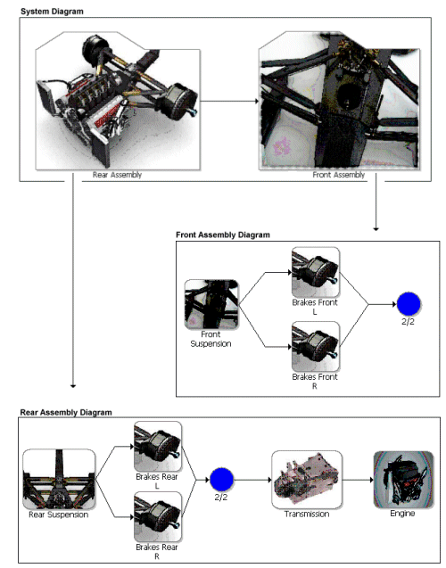
Figure 6: Race Car RBDs

By simulating the operation of the system for 2,000 Km, we obtain the results displayed in Figures 7 and 8. Some of the results of interest include the expected number of system failures (5.104), the total costs ($910,1942), the number of spare parts required for each component, etc.

System-Level Results

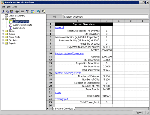
Figure 7: System-Level Results

Component Results

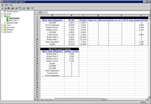
Figure 8: Component Results

The advantages of this approach include the ability to:

Perform criticality and sensitivity analysis.
Identify weak components in the system.
Perform optimization and reliability allocation.
Obtain availability, downtime, expected failures, etc., at the component level as well as the system level.

The main disadvantage is that the analysis requires detailed information, including failure and repair data at the LRU level.

Conclusion

As this article demonstrates, it is not appropriate to analyze a repairable system by applying distribution analysis to interarrival data because time between failure events do not meet the s.i.i.d. requirement. Instead, you may choose to collect data at the system level and analyze it with a stochastic process model, such as the NHPP. Or, you may choose to collect data at the component level and analyze it with a reliability block diagram. Your choice will depend on the data available and the questions you wish to answer based on the analysis.

For more information on the software used to perform the analyses described in this article, visit http://www.reliasoft.com/products/reliability-analysis/weibull, http://www.reliasoft.com/products/reliability-analysis/rga and /content/hbkworld/global/en/products/software/analysis-simulation/reliability/blocksim-system-reliability-availability-maintainability-ram-analysis-software.html.

Main Menu

Main Menu

Main Menu

Main Menu

Avoiding a Common Mistake in the Analysis of Repairable Systems

We have moved ${referer} to www.hbkworld.com

We have moved ${referer} to www.hbkworld.com

We have moved ${referer} to www.hbkworld.com

We have moved ${referer} to www.hbkworld.com

We have moved ${referer} to www.hbkworld.com