Optimum Preventive Maintenance Replacement Time

Maintenance experts agree that replacing a component before it fails (preventively) may, under certain circumstances, make better economic sense than replacing the component when it fails (correctively). The key is to determine whether the preventive replacement of a specific component is appropriate and, if so, to identify the best time to replace the component. This article presents an examination of the simple concept of determining an optimum replacement time for a single component. (Note that although the term "component" is used throughout this article, the principles also apply to replacement decisions concerning subassemblies and assemblies.)

Should a Component be Replaced Preventively?

Two requirements must be met in order for the preventive replacement of a component to be appropriate. First, preventive maintenance makes sense when the component gets worse with time. In other words, as the component ages, it becomes more susceptible to failure or is subject to wearout. In reliability terms, this means that the component has an increasing failure rate. The second requirement is that the cost of preventive maintenance must be less than the cost of corrective maintenance. If both of these requirements are met, then preventive maintenance is appropriate and an optimum time (minimum cost) at which the preventive replacement should take place can be computed.

Computing the Optimum Replacement Time

Figure 1: Cost per Operating Time Unit vs. Operating Time

To compute the optimum replacement time for a component, the analyst must first have a sense of the behavior of the failure rate of the component. This can be obtained using standard life data analysis techniques to determine the life distribution for the component. In most cases, the Weibull life distribution can be used and can be easily computed using ReliaSoft Weibull++. In the case of the Weibull distribution, if the shape parameter, β, is greater than one, then the failure rate increases with time. This satisfies the first requirement for preventive replacement. (Note that an exponential distribution cannot be used in this formulation since the exponential distribution has a constant failure rate). The second requirement to justify preventive replacement depends on the component and can be satisfied if the cost of a planned or preventive replacement (C_P) is less than the cost of an unplanned or corrective replacement (C_U).

If both of these requirements are satisfied, then the cost per operating unit of time vs. operating time can be plotted. In this plot (shown in Figure 1), it can be seen that the corrective replacement costs will increase as time increases (since the   component's failure rate, and thus likelihood of failure, increases with time). The preventive replacement costs will decrease as the time interval increases because the more time passes, the fewer preventive replacement actions will need to be performed. The total cost will be the sum of these two costs. At one point (time t), a minimum cost point exists that determines the optimum preventive replacement time for the component.

The results of the graph are best explained by the following mathematical formulation:

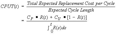
Where C_P is the cost for each preventive action, C_U is the cost for each unplanned or corrective action, and R(t) is the reliability function of the component. The optimum replacement time can be easily obtained by solving for t such that:

Example

For example, consider the simple case of a component following a Weibull distribution with a shape parameter (β) of 2.5 and a scale parameter (η) of 1,000 hours. If we assume a corrective replacement cost of $5 and a preventive replacement cost of $1, the minimum cost (optimum) replacement time for this component would be at 493 hours, with a cost per hour of $0.003462. This is shown graphically in Figure 2.

ReliaSoft BlockSim and Weibull++ software applications include tools for performing this type of analysis.

Figure 2: Optimum Replacement Policy Plot