Using statistical techniques to validate field test data for fatigue analysis

This paper describes some statistical techniques for taking measured data and projecting what the expected time history and resulting fatigue damage would be if test data were collected for much longer times.

Explode view of electric vehicle chassis equipped with battery pack on the road. 3D rendering image.

Table of content

Abstract
Background
Rainflow Reconstruction
Summary

Abstract

During every field test the test engineer is faced with a decision about when sufficient data has been collected to characterize a particular operation. This paper describes some statistical techniques for taking measured data and projecting what the expected time history and resulting fatigue damage would be if test data were collected for much longer times. Sufficient data has been collected when the fatigue damage computed from both the measured and the expected time histories converge.

Background

A major factor in the design of a vehicle or structure is the anticipated severity of the service usage. In a new vehicle, the service usage is unknown and short term tests are frequently conducted to determine the loads acting on the structure and the resulting stresses. The loading history for a vehicle frequently contains both a deterministic and random part. For example, a dump truck may have a deterministic duty cycle of being loaded and unloaded combined with a series of random loads from driving over various surfaces. One may consider the duty cycle loads as variable in nature as well but from a different population than the driving loads. One problem facing all test engineers is to determine when they have collected enough data to characterize a particular service usage condition. Figure 1 shows a measured field loading history for the vertical front suspension loads for an all terrain vehicle ( ATV ) over a test track. The history was recorded for ten laps.

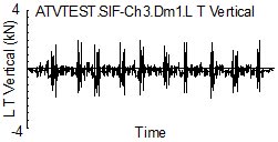Figure 1. Ten laps of test track Despite being a carefully controlled test track and a single driver, the variability in loading during each lap is easily seen in the figure. From a fatigue damage perspective, is the data in Fig. 1 enough to characterize the service usage for the expected life of the component? This question can be answered by using the variability in the measured loading history to project what the expected fatigue damage and loading history would be if the loads were measured for longer time. Analyzing the variability in the time domain for functions of load and time is not feasible or needed. In fatigue, the rainflow histogram of the loads is of more interest than the loading history itself since fatigue damage is computed from it.

Figure 2. Rainflow histogram Two dimensional rainflow histograms contain information about both the load ranges and means. Figure 2 shows the rainflow histogram of the data from Fig. 1 in a To-From format. This type of histogram preserves mean stress effects which are usually important for fatigue analysis. Data from Fig. 2 is plotted as a cumulative exceedance diagram in Fig. 3.

Figure 3. Exceedance diagram The exceedance curve for the original loading history is shown on the left side of the diagram. If the test data were measured for 1000 laps (100 times longer), the distribution would be expected to be shifted to the right and have a similar shape. The dashed lines schematically show that higher loads would be expected for longer times. Although the exceedance diagram is easier to visualize, it looses valuable information about mean effects. In this paper we show how the variability in a measured rainflow histogram can be used to estimate the expected rainflow histogram for longer times. This extrapolated histogram can then be used to reconstruct a new longer time history for testing or analysis. Rainflow Extrapolation Extrapolation of rainflow histograms was first proposed by Dressler [1]. A short description of the concept is given here. Readers are referred to reference 1 for the details. The rainflow histogram is treated as a two dimensional probability distribution. A simple probability density function could be obtained by dividing the number of cycles in each bin of the histogram by the total number of cycles. A new histogram corresponding to any number of total cycles can be constructed by randomly placing cycles in the histogram according to their probability of occurrence. However, this approach will be essentially the same as multiplying the cycles in the histogram by an extrapolation factor. But this is unrealistic. Even the same driver over the same test track cannot repeat the loading history. For example each time a driver hits a pot hole the loads will be somewhat different. This is clearly shown in the ten laps in Fig. 1. The peak load from a particular event will be placed into an individual bin in the rainflow histogram. During subsequent laps, this load will have a different maximum value and be placed into a bin in the same neighborhood as the first lap.

Figure 4. Histogram variability Figure 4 shows a rainflow histogram in a two dimensional view. Consider the event going from 2 to –2.5. Next time this is repeated it will be somewhere in the neighborhood of ( 2, -2.5 ) indicated by the large dashed circle. There is not much data in this region of the histogram and considerable variability is expected. Next consider the cycles from –2 to –1.5. Here there is much more data and we would expect the variability to be much smaller as indicated by the small dashed circle. Extrapolating rainflow histograms is essentially a task of finding a two dimensional probability distribution function from the original rainflow data. For a given set of data taken from a continuous population, X, there are many ways to construct a probability distribution of the data. There are two general classes of probability density estimates: parametric and non-parametric. In parametric density estimation, an assumption is made that the given data set will fit a pre-determined theoretical probability distribution. The shape parameters for the distribution must be estimated from the data. Non-parametric density estimators make no assumptions about the distribution of the entire data set. A histogram is a non-parametric density estimator. For extrapolation purposes, we wish to convert the discrete points of a histogram into a continuous probability density. Kernal estimators [2-3] provide a convenient way to estimate the probability density. The method can be thought of as fitting an assumed probability distribution to a local area of the histogram. The size of the local area is determined by the bandwidth of the estimator. This is indicated by the size of the circle in Fig. 4. An adaptive bandwidth for the kernal is determined by how much data is in the neighborhood of the point being considered. Statistical methods are well developed for regions of the histogram where there is a lot of data. Special considerations are needed for sparsely populated regions [4]. The expected maximum load range for the extrapolated histogram is estimated from a weibull fit to the large amplitude load ranges. This estimate is then used to determine an adaptive bandwidth for the sparse data regions of the histogram. Once the adaptive bandwidth is determined, the probability density of the entire histogram can be computed. The expected histogram for any desired total number of cycles is constructed by randomly placing cycles in the histogram with the appropriate probability. It should be noted that this process does not produce a unique extrapolation. Many extrapolations can be done with the same extrapolation factor so some information about the variability of the resulting loading history can be obtained. Results for a 1000 times extrapolation of the loading history are shown in Fig. 5. It is easier to visualize the results of the extrapolation when the results are viewed in terms of the exceedance diagram given in Fig. 6. Two plots are shown in the figure. One from the data in Fig. 5 and another one representing a 1000 repetitions of the original loading history.

Figure 5. Extrapolated histogram Table 1 gives the results of fatigue lives computed from various extrapolations of the original loading history. Fatigue lives represent the expected operating life of the structure in hours. A simple SN approach was employed in the calculations. Any convenient fatigue analysis technique may be used and can be combined with a probabilistic description of the material properties. Table 1. Fatigue Lives

History	Life	Maximum	Minimum
Original	29,890	1.89	-2.12
10X	26,760	2.25	-2.50
100X	16,170	2.88	-3.25
1000X	10,190	3.25	-3.63

As expected, computed fatigue lives are lower for longer loading histories because of the higher loads in the extrapolated histograms. But the higher loads represent a more realistic forecast of the operating loads during the entire lifetime of the structure.

Figure 6. Distribution of cycles and fatigue damage One effective method to visualize the damaging cycles is to plot the distribution of cycles and material behavior on the same scale as shown in Fig. 6. Material properties are scaled so that they have the same units as the loading history and this plot represents the expected fatigue life under constant amplitude loading. The point of tangency of the two curves gives an indication of the most damaging range of cycles. The maximum load range cycles are not the most damaging in this history, rather the most damaging cycles for this loading history are at about ½ of the maximum load range in the extrapolated histogram.

Rainflow Reconstruction

The objective of rainflow reconstruction is to obtain a time history that will have similar fatigue damage as the original rainflow histogram[5]. In essence, we wish to perform rainflow counting backwards. Starting with the rainflow histogram, reconstruct a time history, cycle by cycle, that has the same rainflow count. The largest overall cycle in the histogram is known. In the To-From format, rainflow counting distinguishes the difference between a Peak-Valley-Peak (PV) cycle and a Valley-Peak-Valley (VP) cycle. VP cycles are stored above the principle diagonal of the histogram and PV cycles below. The row of the histogram is less than the column for any VP cycle. Similarly, the column is less than the row for any PV cycle. The process for inserting VP cycles is illustrated in Fig. 7. The numbers on the left indicate histogram bins, row or column, and are proportional to the magnitude of the resulting loading history. The reconstructed time history is denoted P and V and the cycle to be inserted is denoted as r and c.

Figure 7. Inserting a VP cycle An VP cycle ( r < c ) can be inserted into any PV reversal if c <= P and r > V. A VP cycle can not be inserted into a PV cycle of the same magnitude.

Figure 8. Insertion of a PV cycle Figure 8 shows the insertion of a PV cycle. An PV cycle ( c < r ) can be inserted into any VP reversal if r < P and c >= V. A PV cycle can not be inserted into a VP cycle of the same magnitude. These two simple rules provide the basis for rainflow reconstruction. The process starts with the largest cycle either PVP or VPV. The next largest cycle is then inserted in an appropriate location in the reconstructed time history. After the first few cycles, there are many possible locations to insert a smaller cycle. All possible insertion locations are determined and one is selected at random.

Summary

Reliability of a vehicle or structure is influenced by the distribution of loading during the entire service usage. A technique for estimating the long term durability from short term measured loads has been described.

References

[1] Dressler, K, B. Grunder, M. Hack and V.B. Koettgen, "Extrapolation of rainflow matrices", SAE Paper 960569, 1996
[2] Silverman, B.W. "Density estimation for statistics and data analysis" Chapman and Hall, New York, 1986
[3] Scott, D.W. "Multivariate density estimation" Wiley, New York, 1992
[4] Roth, J.S. "Statistical modeling of rainflow histograms" Materials Engineering-Mechanical Behavior Report No. 182, UILU-ENG 98-4017, University of Illinois, 1998
[5] Khosrovaneh, A.K. and N.E. Dowling, "Fatigue loading history reconstruction based on the rainflow technique", International Journal of Fatigue, Vol. 12, No. 2, 1990, 99-106

Main Menu

Main Menu

Main Menu

Main Menu

Using statistical techniques to validate field test data for fatigue analysis

Table of content

Abstract

Background

Rainflow Reconstruction

Summary

References

We have moved ${referer} to www.hbkworld.com

We have moved ${referer} to www.hbkworld.com

We have moved ${referer} to www.hbkworld.com

We have moved ${referer} to www.hbkworld.com

We have moved ${referer} to www.hbkworld.com

We haved moved ${referer} to www.hbkworld.com