[Please note that the following article — while it has been updated from our newsletter archives — may not reflect the latest software interface and plot graphics, but the original methodology and analysis steps remain applicable.]
When performing reliability growth analysis during the in-house developmental testing of a product, it is common practice to use non-homogeneous Poisson process (NHPP) models (such as the Crow-AMSAA) to model failure data. The assumption of these models is that the failure intensity is monotonically increasing, decreasing or remaining constant over time. However, there might be cases in which the system design or the operational environment experiences major changes during the observation period and a single model will not be appropriate to describe the failure behavior for the entire timeline.
In this article, we will present a methodology that can be applied to scenarios in which a major change occurs during a reliability growth test. We will show how the test data can be broken into two segments with a separate Crow-AMSAA (NHPP) model applied to each segment. We will also provide an example that shows how this methodology can be applied using ReliaSoft RGA software. First, we will give a brief overview of the Crow-AMSAA (NHPP) model.
The Crow-AMSAA (NHPP) is one of the most popular models used for modeling time-to-failure data obtained during developmental testing. Under this model, failures occur according to a non-homogeneous Poisson process with a Weibull intensity function. The failure intensity function is:
![]()
where:
The cumulative number of failures under the Crow-AMSAA (NHPP) model is given by:

By taking the logarithmic transformation of both sides, the above equation can be linearized as:
![]()
Therefore, in the Crow-AMSAA (NHPP) model, the cumulative number of failures versus the cumulative test time is linear on logarithmic scales.
The parameters of the model, β and λ, are calculated using maximum likelihood estimation (MLE) methods. The ML estimators for the two parameters are:

where:
Consider the data in Figure 1 that were obtained during a reliability growth test. As discussed above, the cumulative number of failures vs. the cumulative time should be linear on logarithmic scales.
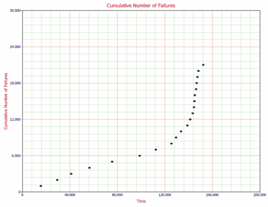
Figure 1: Cumulative number of failures from reliability growth test
Figure 2 shows the data plotted on logarithmic scales. One can easily recognize that the failure behavior is not constant throughout the duration of the test. Just by observing the data, it can be asserted that a major change occurred at around 140 hours that resulted in a change in the rate of failures. Therefore, using a single model to analyze this data set may not be appropriate.
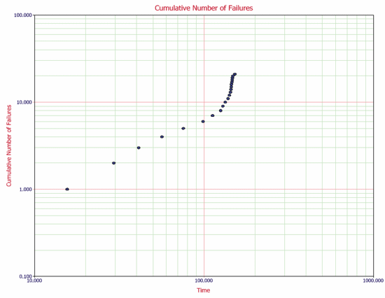
Figure 2: Cumulative number of failures plotted on logarithmic axes
The "Change of Slope" methodology proposes to split the data into two segments and apply a Crow-AMSAA (NHPP) model to each segment. The time that will be used to split the data into the two segments (it will be referred to as T1) could be estimated just by observing the data but will most likely be dictated by engineering knowledge of the specific change to the system design or operating conditions. It is important to note that although two separate models will be applied to the segments, the information collected in the first segment (i.e., data up to T1) will be considered when creating the model for the second segment (i.e., data after T1). The models presented next can be applied to the reliability growth analysis of a single system or multiple systems. [1]
The data up to the point of the change that occurs at T1 will be analyzed using the Crow-AMSAA (NHPP) model. The ML estimators of the model are:

where:
The Crow-AMSAA (NHPP) model will be used again to analyze the data after T1. However, the information collected during the first segment will be used when creating the model for the second segment. Given that, the ML estimators of the model parameters in the second segment are:

where:
Table 1 gives the failure times obtained from a reliability growth test of a newly designed system.
Table 1: Failure times from a reliability growth test
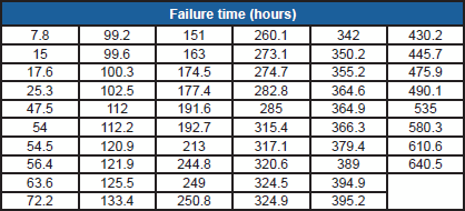
The test has a duration of 660 hours and Figure 3 shows the plot of the cumulative number of failures over time on logarithmic scales.
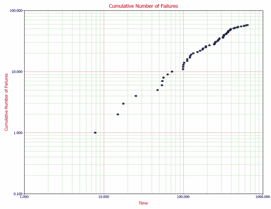
Figure 3: Cumulative number of failures over time on logarithmic scales for data in Table 1
First, let us try to apply a single model to all of the data. The Crow-AMSAA (NHPP) model is chosen for that purpose. Figure 4 shows the expected failures obtained from the model (the line) along with the observed failures (the points). As it can be seen from the plot, the model does not seem to accurately track the data. That is confirmed by performing the Cramér-von Mises goodness-of-fit test, which checks the hypothesis that the data follows a non-homogeneous Poisson process with a power law failure intensity. (For more details, see [2].) The model fails the goodness-of-fit test because the test statistic (0.3309) is higher than the critical value (0.1729) at the 0.1 significance level. Figure 4 also shows a customized report that displays both the calculated parameters and the statistical test results.
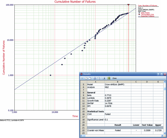
Figure 4: Analysis of the entire data set with a single Crow-AMSAA (NHPP) model
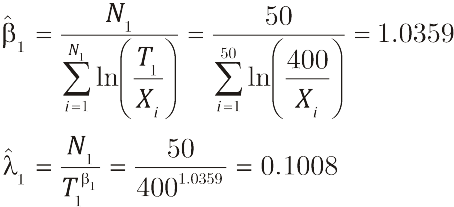
Through further investigation, the analysts discover that a significant design change occurred at 400 hours of test time and they suspect this modification is responsible for the change in the failure behavior. They decide to apply the "Change of Slope" methodology and break the data into two segments. The first segment is set from 0 to 400 hours and the second segment is from 401 to 660 hours (which is the end time of the test). The Crow-AMSAA (NHPP) parameters for the first segment (0-400 hours) are:
The Crow-AMSAA (NHPP) parameters for the second segment (401-660 hours) are:
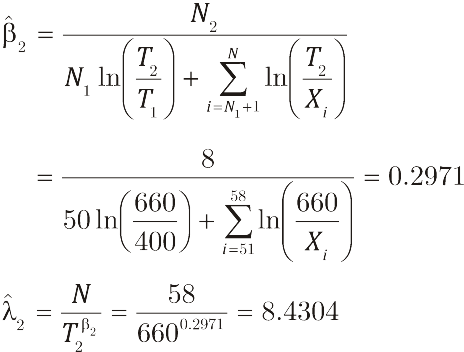
Figure 5 shows a plot of the two-segment analysis along with the observed data. It is obvious that the "Change of Slope" method tracks the data more accurately. This can also be verified by performing a goodness-of-fit test. In this case, a Chi-Squared test will be applied because it is appropriate for grouped data and the "Change of Slope" method uses grouped data analysis for the second segment. (For more details, see [2]). The Chi-Squared statistic for this analysis is 1.2956, which is lower than the critical value of 12.017 at the 0.1 significance level; therefore, the analysis passes the test. Figure 5 also shows a customized report that displays both the calculated parameters and the statistical test results.
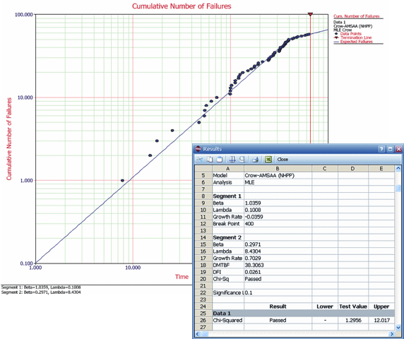
Figure 5: Analysis based on the "Change of Slope" methodology with two Crow-AMSAA (NHPP) models
Now that we have a model that fits the data, we can use it to make accurate predictions and calculations. We can calculate metrics such as the demonstrated MTBF at the end of the test or the expected number of failures at later times. For example, Figure 6 shows the demonstrated MTBF (i.e., the instantaneous MTBF at the end of the test) and the plot of MTBF vs. Time. The parameters of the first segment were used to calculate the MTBF for times up to 400 hours; while the parameters of the second segment were used for times after 400 hours.
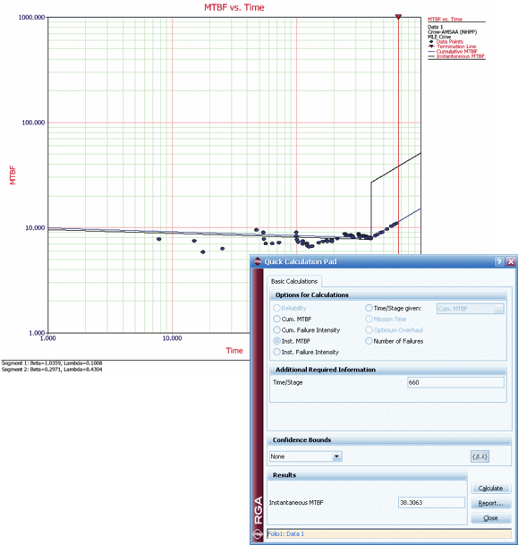
Figure 6: Demonstrated MTBF at the end of the test (660 hours) and plot of the MTBF vs. Time
In this article, we have presented the "Change of Slope" methodology that can be used for analyzing reliability growth data when a major change has occurred during the test that affects the failure behavior. We have shown that applying a single model in such situations is not appropriate for accurate predictions. Instead, the "Change of Slope" methodology splits the data into two segments and applies a Crow-AMSAA (NHPP) model to each segment, where the information collected during the first segment is considered when modeling the second segment. As a result, the overall data set is modeled more accurately and better predictions and metric calculations can be obtained.
[1] Guo, H., Mettas, A., Sarakakis, G. and Niu P., "Piecewise NHPP Models with Maximum Likelihood Estimation for Repairable Systems," Proceedings of the Annual Reliability and Maintainability Symposium, 2010.
[2] ReliaSoft, Reliability Growth & Repairable Systems Data Analysis Reference, ReliaSoft Publishing, 2009.